plenoptic.plot.imshow

plenoptic.plot.imshow(image, vrange='indep1', zoom=None, title='', col_wrap=None, ax=None, cmap=None, plot_complex='rectangular', batch_idx=None, channel_idx=None, as_rgb=False, **kwargs)

Show image(s), avoiding interpolation.

This function shows images carefully, avoiding interpolation: each element in the input image will correspond to a pixel or an integer number of pixels. When zoom<1, an integer number of input elements will be averaged into a single pixel.

Parameters:

• image (Tensor | list[Tensor]) – The images to display. Tensors should be 4d (batch, channel, height, width). List of tensors should be used for tensors of different height and width: all images will automatically be rescaled so they’re displayed at the same height and width, thus, their heights and widths must be scalar multiples of each other.

• vrange (tuple[float, float] | str (default: 'indep1')) –

  If a 2-tuple, specifies the image values vmin/vmax that are mapped to the minimum and maximum value of the colormap, respectively. If a string:

  • "auto0": All images have same vmin/vmax, which have the same absolute value, and come from the minimum or maximum across all images, whichever has the larger absolute value.

  • "auto1": All images have same vmin/vmax, which are the minimum/maximum values across all images.

  • "auto2": All images have same vmin/vmax, which are the mean (across all images) minus/ plus 2 std dev (across all images).

  • "auto3": All images have same vmin/vmax, chosen so as to map the 10th/90th percentile values to the 10th/90th percentile of the display intensity range. For example: vmin is the 10th percentile image value minus 1/8 times the difference between the 90th and 10th percentile.

  • "indep0": Each image has an independent vmin/vmax, which have the same absolute value, which comes from either their minimum or maximum value, whichever has the larger absolute value.

  • "indep1": Each image has an independent vmin/vmax, which are their minimum/maximum values.

  • "indep2": Each image has an independent vmin/vmax, which is their mean minus/plus 2 std dev.

  • "indep3": Each image has an independent vmin/vmax, chosen so that the 10th/90th percentile values map to the 10th/90th percentile intensities.

• zoom (float | None (default: None)) – Ratio of display pixels to image pixels. If greater than 1, must be an integer. If less than 1, must be 1/d where d is a a divisor of the size of the largest image. If None, we try to determine the best zoom.

• title (str | list[str] | None (default: '')) –

  Title for the plot. In addition to the specified title, we add a subtitle giving the plotted range and dimensionality (with zoom).

  • If str, will put the same title on every plot.

  • If list, all values must be str, must be the same length as img, and each title will be assigned to corresponding plot.

  • If None, no title will be printed and subtitle will be removed.

• col_wrap (int | None (default: None)) – Number of axes to have in each row. If None, will fit all axes in a single row.

• ax (Axes | None (default: None)) – If None, we make the appropriate figure. Otherwise, we shrink the axes so that it’s the appropriate number of pixels.

• cmap (Colormap | None (default: None)) – Colormap to use when showing these images. If None, then behavior is determined by vrange: if vmap in ["auto0", "indep0"], we use "RdBu_r", else we use "gray" (see matplotlib documentation).

• plot_complex (Literal['rectangular', 'polar', 'logpolar'] (default: 'rectangular')) –

  Specifies handling of complex values.

  • "rectangular": plot real and imaginary components as separate images.

  • "polar": plot amplitude and phase as separate images.

  • "logpolar": plot log (base 2) amplitude and phase as separate images.

• batch_idx (int | None (default: None)) – Which element from the batch dimension to plot. If None, we plot all.

• channel_idx (int | None (default: None)) – Which element from the channel dimension to plot. If None, we plot all. Note if this is not None, then as_rgb=True will fail, because we restrict the channels.

• as_rgb (bool (default: False)) – Whether to consider the channels as encoding RGB(A) values. If True, we attempt to plot the image in color, so your tensor must have 3 (or 4 if you want the alpha channel) elements in the channel dimension. If False, we plot each channel as a separate grayscale image.

• **kwargs (Any) – Passed to matplotlib.pyplot.imshow.

Return type:

PyrFigure

Returns:

fig – Figure containing the plotted images.

Raises:

• ValueError – If images is not a 4d tensor or list of 4d tensors.

• TypeError – If batch_idx or channel_idx are not an int or None.

• IndexError – If batch_idx or channel_idx are out of bounds.

• ValueError – If zoom takes an illegal value.

• ValueError – If as_rgb=True and the input image does not have 3 or 4 channels.

• ValueError – If as_rgb=False, image has more than one channel and one more than one batch and neither batch_idx nor channel_idx is set.

• Exception – If plot_complex takes an illegal value.

See also

synthesis_imshow

Show the image synthesized by a synthesis object.

animshow

Animate a video.

pyrshow

Display steerable pyramid coefficients.

Notes

This interpolation avoidance is only guaranteed for the saved image; it should generally hold in notebooks as well, but will fail if, e.g., you plot an image that’s 2000 pixels wide on an monitor 1000 pixels wide; the browser handles the rescaling in a way we can’t control.

Examples

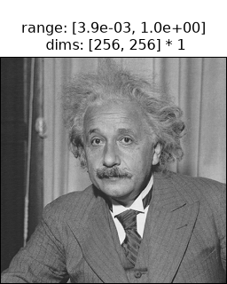
Plot a single grayscale image:

>>> import plenoptic as po
>>> einstein = po.data.einstein()
>>> einstein.shape
torch.Size([1, 1, 256, 256])
>>> po.plot.imshow(einstein)
<PyrFigure size ... with 1 Axes>

(png, hires.png, pdf)

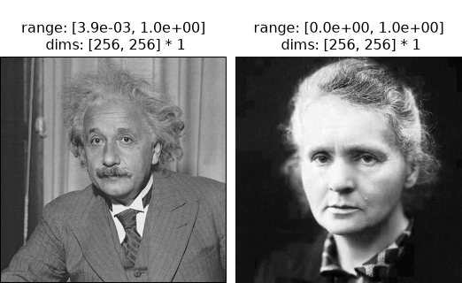
For an image tensor with multiple elements along the batch dimension and a single channel element, this function will plot each batch independently as grayscale images:

>>> import torch
>>> curie = po.data.curie()
>>> imgs = torch.cat([einstein, curie])
>>> print(imgs.shape)
torch.Size([2, 1, 256, 256])
>>> po.plot.imshow(imgs)
<PyrFigure size ... with 2 Axes>

(png, hires.png, pdf)

A list of 4d tensors will be concatenated along the batch dimension before plotting. Thus, the following example is the same as above:

>>> po.plot.imshow([einstein, curie])
<PyrFigure size ... with 2 Axes>

(png, hires.png, pdf)

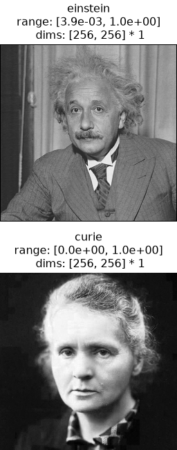
You may use the title argument for any number of images, either as a string applied to all images or as a list the length of images. Additionally, col_wrap specifies the number of images per row:

>>> po.plot.imshow(imgs, title=["einstein", "curie"], col_wrap=1)
<PyrFigure size ... with 2 Axes>

(png, hires.png, pdf)

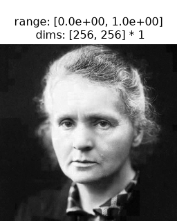
Specifying batch_idx will plot the corresponding element in the batch dimension (i.e., imgs[batch_idx]):

>>> print(imgs.shape)
torch.Size([2, 1, 256, 256])
>>> po.plot.imshow(imgs, batch_idx=1)
<PyrFigure size ... with 1 Axes>

(png, hires.png, pdf)

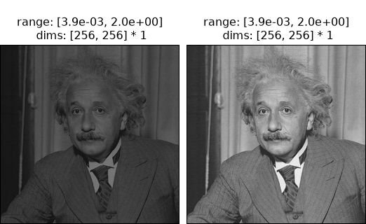
The vrange argument allows control over the min and max values of the color range. In addition to a 2-tuple of floats, this functions accepts several special strings (see docstring for details). For example, "auto1" sets all images to have the same range:

>>> einsteins_scaled = torch.cat([einstein, einstein * 2])
>>> po.plot.imshow(einsteins_scaled, vrange="auto1")
<PyrFigure size ... with 2 Axes>

(png, hires.png, pdf)

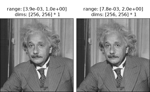
Meanwhile, "indep1" sets each image’s range independently. Note the different ranges in the titles!

>>> po.plot.imshow(einsteins_scaled, vrange="indep1")
<PyrFigure size ... with 2 Axes>

(png, hires.png, pdf)

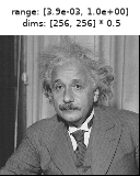
The zoom argument allows users to set the ratio of display to image pixels, increasing or decreasing the size of the resulting plot:

>>> po.plot.imshow(einstein, zoom=0.5)
<PyrFigure size ... with 1 Axes>

(png, hires.png, pdf)

Note that if zoom<1 and the value is not a divisor of the largest image size, this function will raise an error:

>>> print(einstein.shape)
torch.Size([1, 1, 256, 256])
>>> po.plot.imshow(einstein, zoom=0.7)
Traceback (most recent call last):
Exception: zoom * signal.shape must result in integers!

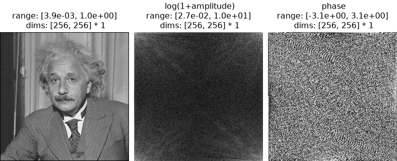
You can use the plot_complex argument to control how complex tensors are plotted:

>>> einstein_fft = torch.fft.fft2(einstein)
>>> po.plot.imshow([einstein, einstein_fft], plot_complex="logpolar")
<PyrFigure size ... with 3 Axes>

(png, hires.png, pdf)

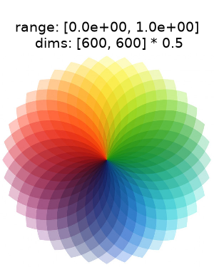
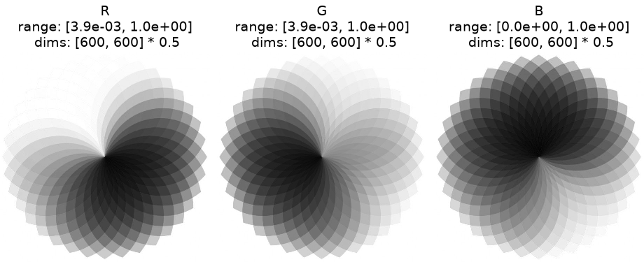
To plot a RGB(A) image in color, you must set as_rgb=True:

>>> color_wheel = po.data.color_wheel()
>>> print(color_wheel.shape)
torch.Size([1, 3, 600, 600])
>>> po.plot.imshow(color_wheel, as_rgb=True, zoom=0.5)
<PyrFigure size ... with 1 Axes>

(png, hires.png, pdf)

Otherwise, images with multiple channels will have each channel plotted as a separate grayscale image:

>>> po.plot.imshow(color_wheel, zoom=0.5, title=["R", "G", "B"])
<PyrFigure size ... with 3 Axes>

(png, hires.png, pdf)

This function will raise a ValueError if as_rgb=True and the input image doesn’t have the required number of channels:

>>> print(einstein.shape)
torch.Size([1, 1, 256, 256])
>>> po.plot.imshow(einstein, as_rgb=True)
Traceback (most recent call last):
ValueError: If as_rgb is True, then channel must have 3 or 4 elements!

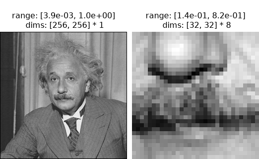
Images will be automatically rescaled to be displayed at the same heights and widths if sizes are scalar multiples of each other:

>>> einstein_cropped = po.process.center_crop(einstein, 32)
>>> po.plot.imshow([einstein, einstein_cropped])
<PyrFigure size ... with 2 Axes>

(png, hires.png, pdf)