plenoptic.plot.synthesis_loss

plenoptic.plot.synthesis_loss(synthesis_object, iteration=None, plot_penalties=False, ax=None, **kwargs)

Plot synthesis loss.

Added in version 2.0: Combines previously separate loss plotting functions for Metamer and MADCompetition, and adds support for plotting penalties. Note that behavior for Metamer is different: we now plot the metamer loss, not the objective function value (see below for details).

The behavior of this function is slightly different depending on the type of synthesis_object:

• Metamer: creates a single axis object whose y-axis is log-scaled and shows the metamer loss and, if plot_penalties=True, penalties. Returned dictionary has key "loss".

• MADCompetition: creates multiple axes objects, one each for reference_metric_loss, optimized_metric_loss, and (if plot_penalties=True) penalties. The y-axis is linearly-scaled for all plots. Returned dictionary has keys "reference_metric_loss", "optimized_metric_loss", and "penalties".

In all cases, plots a red dot at iteration, to highlight the loss there. If iteration=None, then the dot will be at the final iteration.

Attention

In all cases, we plot the components of the objective function, not the objective function itself (whose values are stored in the plenoptic.Metamer.losses or plenoptic.MADCompetition.losses attribute). See Examples section and plenoptic.Metamer.objective_function or plenoptic.MADCompetition.objective_function for more details.

Parameters:

• synthesis_object (Metamer | MADCompetition) – Synthesis object whose loss we want to plot.

• iteration (int | None (default: None)) – Which iteration to display. If None, we show the most recent one. Negative values are also allowed.

• plot_penalties (bool (default: False)) – Whether to plot the output of the penalty function as well. See above for behavior.

• ax (list[Axes] | Axes | None (default: None)) – Pre-existing axes for plot. If None, we call matplotlib.pyplot.gca. If synthesis_object is MADCompetition, then if ax is a single axis, we split it horizontally; if ax is a list, it must contain two (or three, if plot_penalties=True) axes to plot on. If synthesis_object is Metamer, then passing a list will result in a ValueError.

• **kwargs (Any) – Passed to matplotlib.pyplot.plot.

Return type:

dict[str, Axes]

Returns:

axes_dict – A dictionary whose keys are strings describing the created plots and whose values are the corresponding matplotlib axes. See above for details.

Raises:

• IndexError – If iteration takes an illegal value.

• ValueError – If ax is a list and synthesis_object is a Metamer.

• ValueError – If synthesis_object is a MADCompetition and ax is a list of the wrong length.

• TypeError – If synthesis_object is not MADCompetition or Metamer

See also

synthesis_status

Create a figure combining this with other axis-level plots to summarize synthesis status at a given iteration.

synthesis_animate

Create a video animating this and other axis-level plots changing over the course of synthesis.

Examples

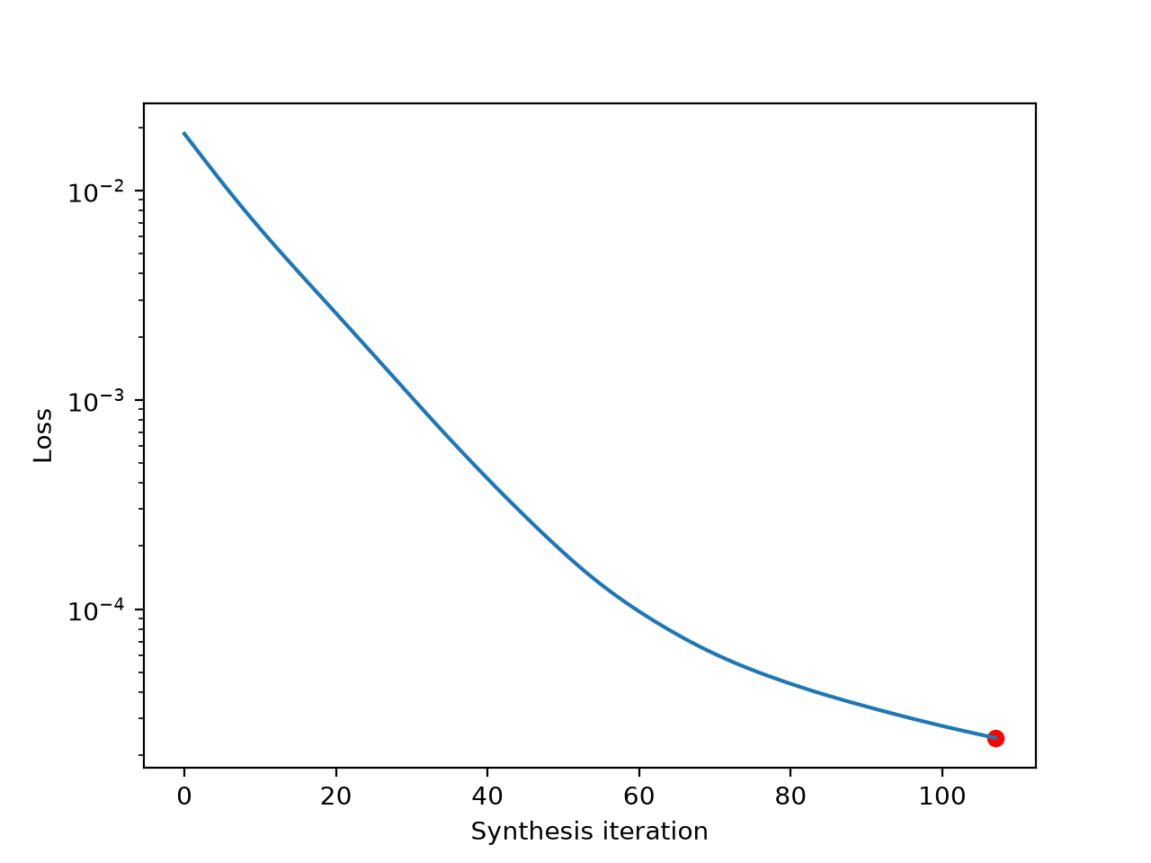
Plot loss for Metamer object:

>>> import plenoptic as po
>>> import matplotlib.pyplot as plt
>>> import torch
>>> img = po.data.einstein()
>>> model = po.models.Gaussian(30).eval()
>>> po.remove_grad(model)
>>> met = po.Metamer(img, model)
>>> met.to(torch.float64)
>>> met.load(po.data.fetch_data("example_metamer_gaussian.pt"))
>>> po.plot.synthesis_loss(met)
{'loss': <Axes: ... ylabel='Loss'>}

(png, hires.png, pdf)

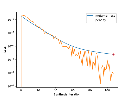
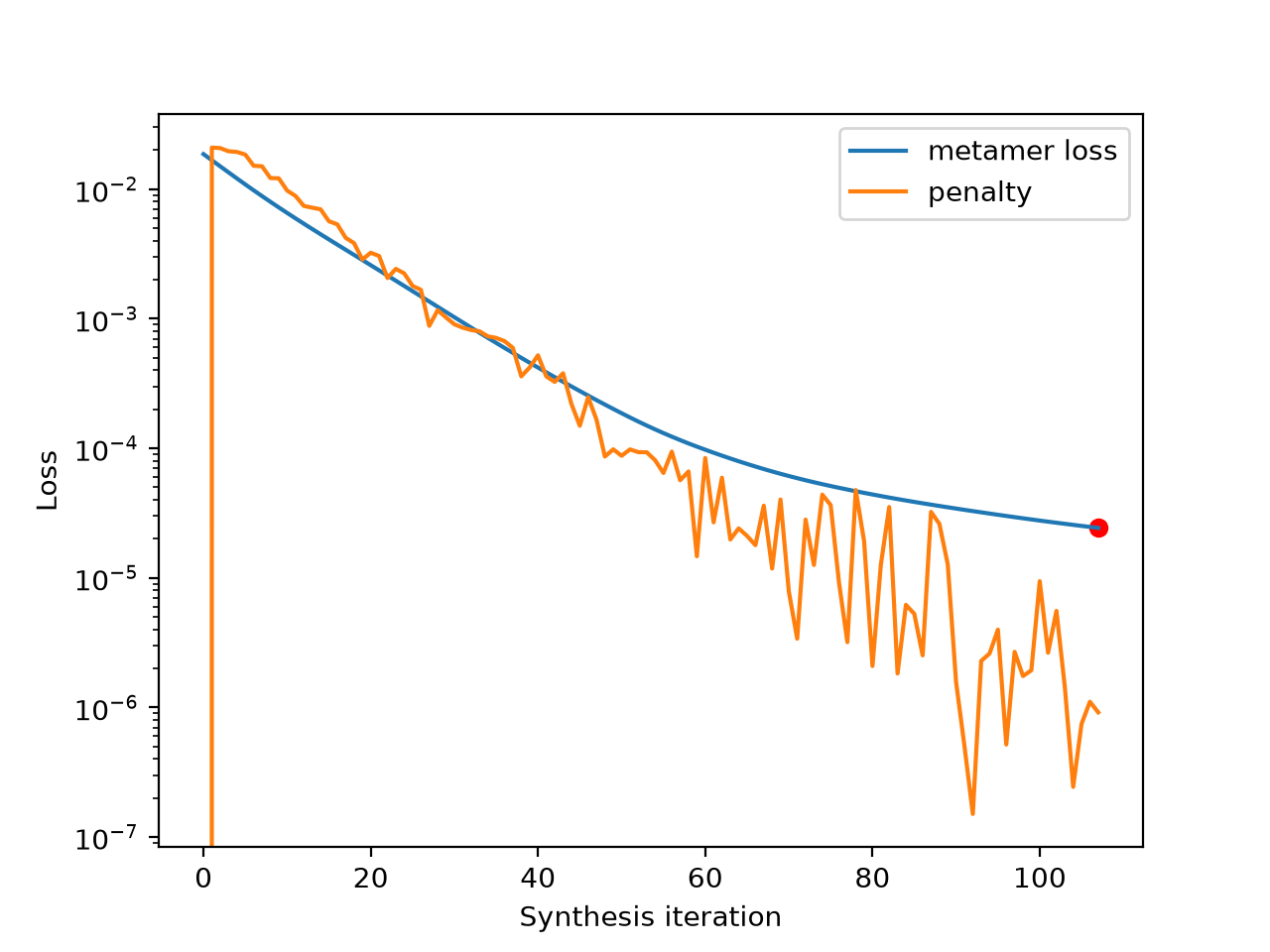
Include the penalties:

>>> po.plot.synthesis_loss(met, plot_penalties=True)
{'loss': <Axes: ... ylabel='Loss'>}

(png, hires.png, pdf)

Specify an iteration:

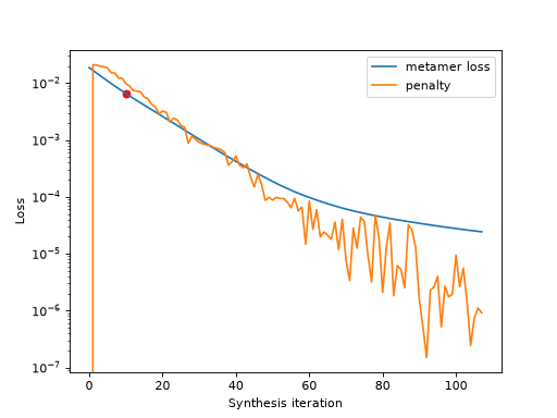
>>> po.plot.synthesis_loss(met, iteration=10, plot_penalties=True)
{'loss': <Axes: ... ylabel='Loss'>}

(png, hires.png, pdf)

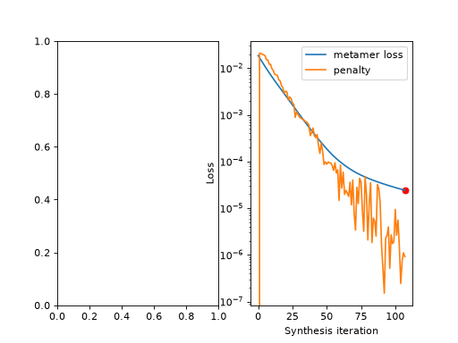
Plot on an axis in an existing figure:

>>> fig, axes = plt.subplots(1, 2)
>>> po.plot.synthesis_loss(met, ax=axes[1], plot_penalties=True)
{'loss': <Axes: ... ylabel='Loss'>}

(png, hires.png, pdf)

Note that we are not plotting the output of plenoptic.Metamer.objective_function, which is stored in plenoptic.Metamer.losses. Instead, we are plotting the output of plenoptic.Metamer.loss_function, which is the “metamer loss” (which does not include the penalty). The following example illustrates the difference:

>>> axes = po.plot.synthesis_loss(met)
>>> axes["loss"].plot(met.losses, label="objective function")
[<matplotlib.lines.Line2D ...>]
>>> # Some tweaks to the marker and size to aid visibility.
>>> axes["loss"].plot(
...     met.losses - met.penalty_lambda * met.penalties,
...     "k.",
...     ms=2,
...     label="reconstructed metamer loss",
... )
[<matplotlib.lines.Line2D ...>]
>>> axes["loss"].legend()
<matplotlib.legend.Legend ...>

(png, hires.png, pdf)

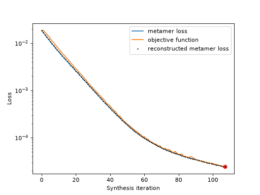
Notice how the objective function line is above the one created by the this function, and how we compute the metamer loss alone.

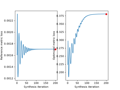
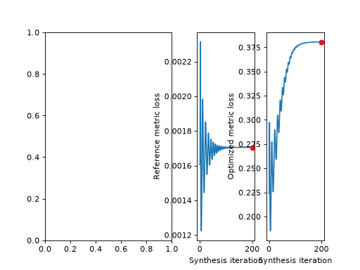
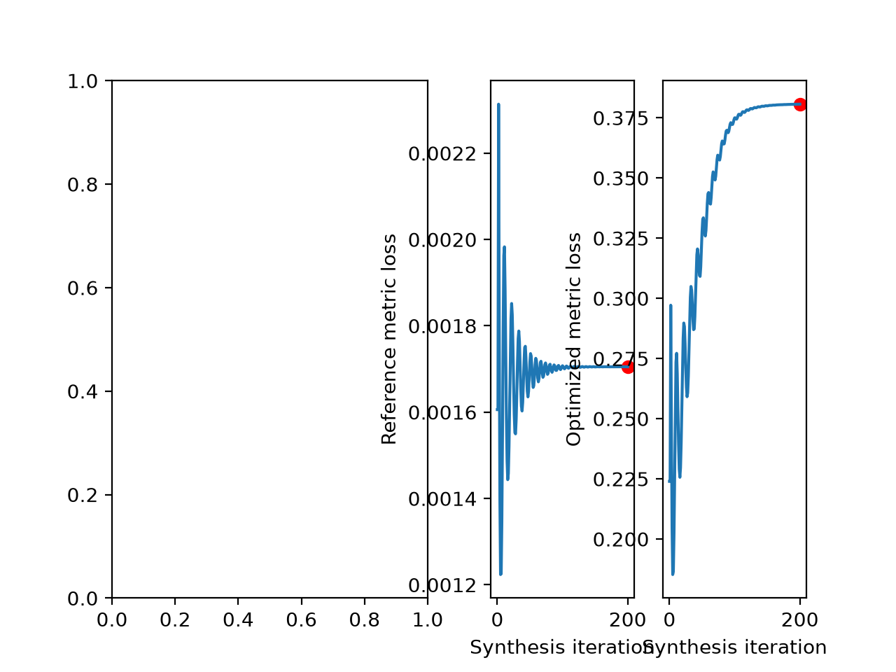
Plot loss for MADCompetition object:

>>> img = po.data.einstein().to(torch.float64)
>>> def ds_ssim(x, y):
...     return 1 - po.metric.ssim(x, y, weighted=True, pad="reflect")
>>> mad = po.MADCompetition(img, ds_ssim, po.metric.mse, "max", 1e6)
>>> mad.load(po.data.fetch_data("example_mad.pt"))
>>> po.plot.synthesis_loss(mad)
{'reference_metric_loss': <Axes: ...>, 'optimized_metric_loss': <Axes: ...>}

(png, hires.png, pdf)

When plotting MADCompetition loss on an existing figure, you can either pass a single axis, in which case we sub-divide it into the necessary number of axes, or a list with the appropriate number of axes:

>>> fig, axes = plt.subplots(1, 2)
>>> po.plot.synthesis_loss(mad, ax=axes[1])
{'reference_metric_loss': <Axes: ...>, 'optimized_metric_loss': <Axes: ...>}
>>> fig, axes = plt.subplots(1, 2)
>>> po.plot.synthesis_loss(mad, ax=axes)
{'reference_metric_loss': <Axes: ...>, 'optimized_metric_loss': <Axes: ...>}

Fig. 9 (png, hires.png, pdf)

Fig. 10 (png, hires.png, pdf)

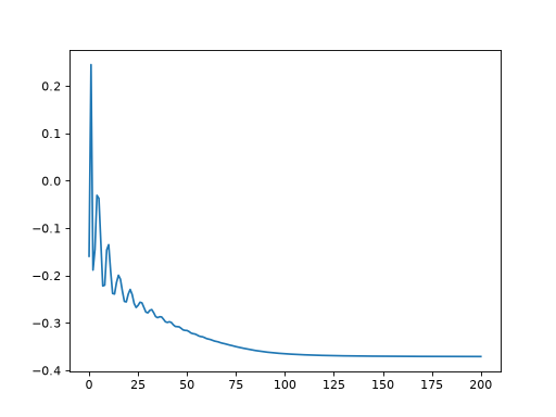
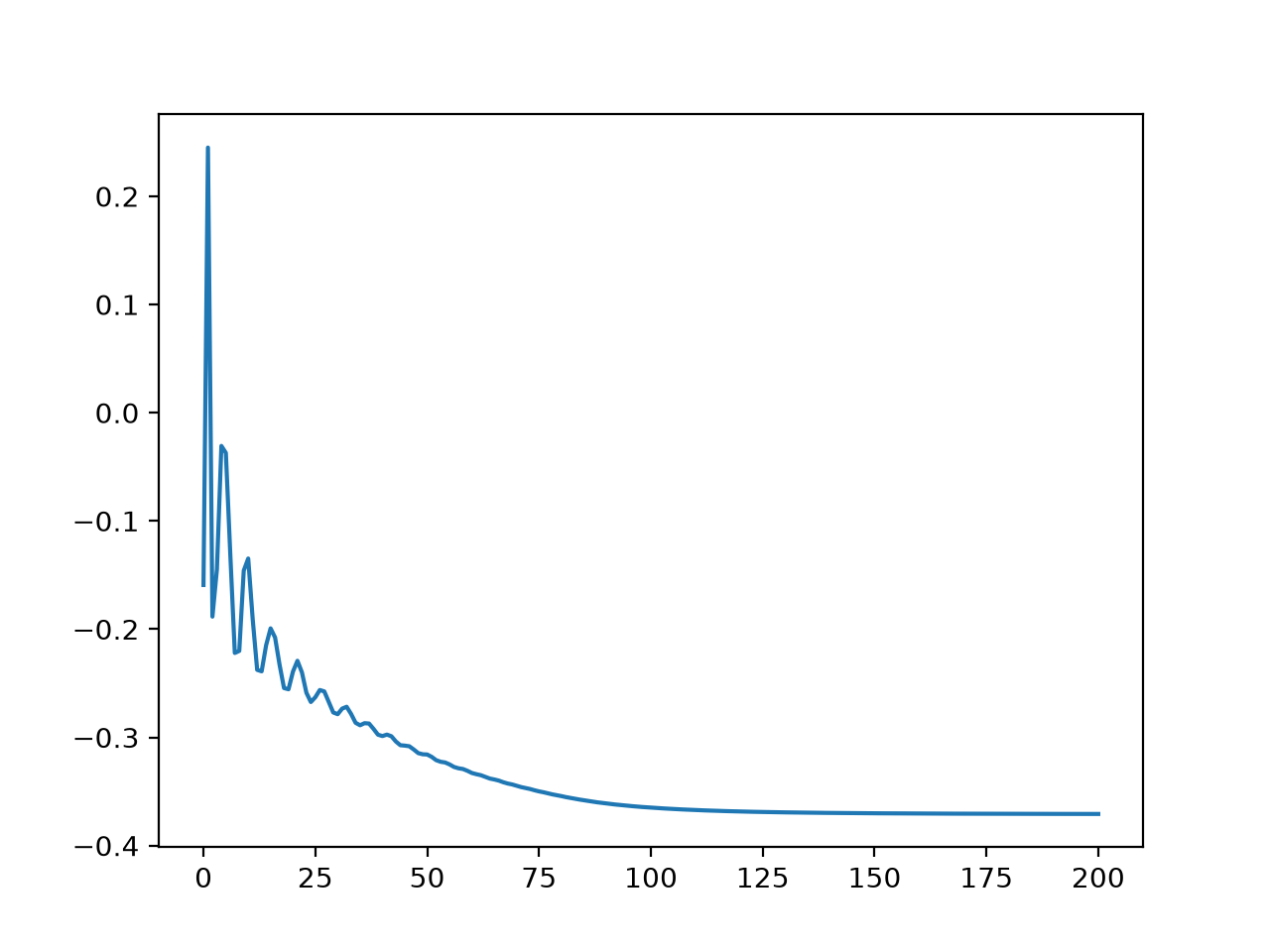
Note that, as with Metamer, we are not plotting the output of plenoptic.MADCompetition.objective_function, which is stored in plenoptic.MADCompetition.losses. Instead, we are plotting the output of the two metrics we are comparing. If you wish to plot the objective function output, you can do so directly:

>>> plt.plot(mad.losses)
[<matplotlib.lines.Line2D ...>]

(png, hires.png, pdf)