plenoptic.process.skew

plenoptic.process.skew(x, mean=None, var=None, dim=None, keepdim=False)

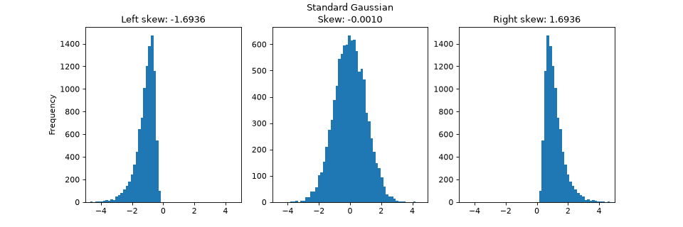
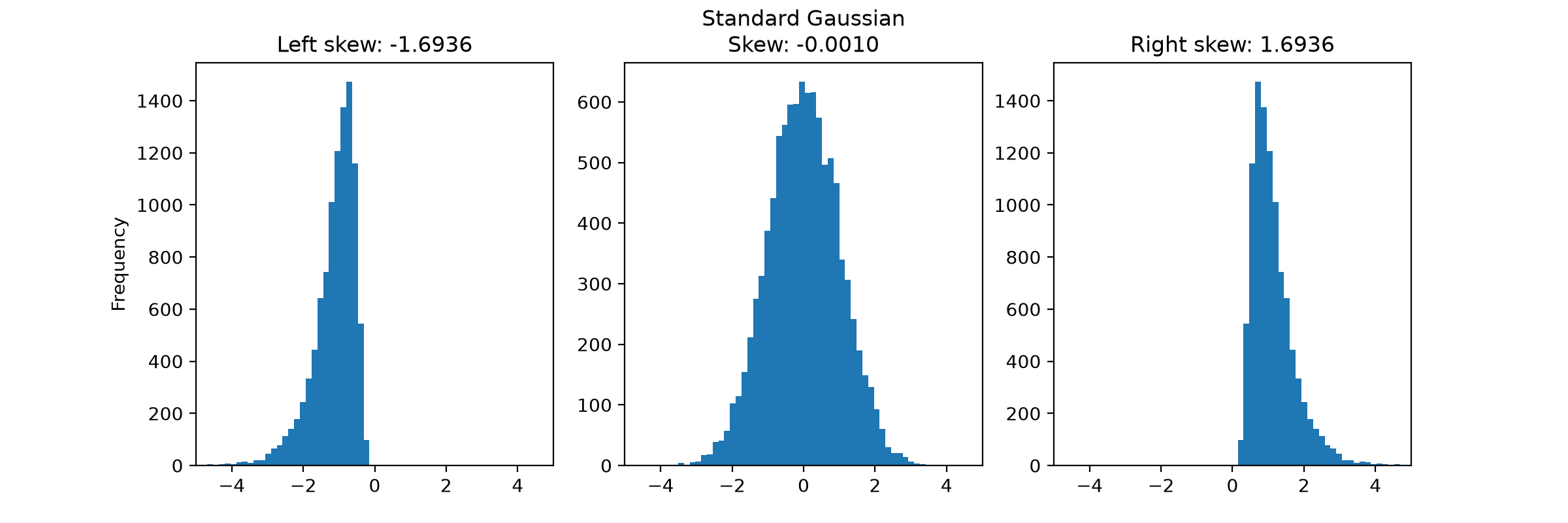
Calculate sample estimate of asymmetry about input’s mean.

To help with interpretation:

• Skew of normal distribution is 0.

• Negative skew, also known as left-skewed: the left tail is longer. Distribution appears as a right-leaning curve.

• Positive skew, also known as right-skewed: the right tail is longer. Distribution appears as a left-leaning curve.

Parameters:

• x (Tensor) – The input tensor.

• mean (float | Tensor | None (default: None)) – Reuse a precomputed mean.

• var (float | Tensor | None (default: None)) – Reuse a precomputed variance.

• dim (int | list[int] | None (default: None)) – The dimension or dimensions to reduce.

• keepdim (bool (default: False)) – Whether to retain the reduced dimensions (as singletons) or not.

Return type:

Tensor

Returns:

out – The skewness tensor.

See also

variance

Calculate sample variance.

kurtosis

Calculate sample kurtosis.

Examples

>>> import plenoptic as po
>>> import matplotlib.pyplot as plt
>>> import torch
>>> po.set_seed(42)
>>> x = torch.randn(10000)
>>> s = po.process.skew(x)
>>> x_right = torch.exp(x / 2)
>>> s_right = po.process.skew(x_right)
>>> x_left = -torch.exp(x / 2)
>>> s_left = po.process.skew(x_left)
>>> fig, (ax_left, ax, ax_right) = plt.subplots(
...     1, 3, sharex=True, figsize=(12, 4)
... )
>>> _ = ax_left.hist(x_left, bins=50)
>>> _ = ax_left.set(
...     title=f"Left skew: {s_left:.4f}", ylabel="Frequency", xlim=(-5, 5)
... )
>>> _ = ax.hist(x, bins=50)
>>> _ = ax.set(title=f"Standard Gaussian\nSkew: {s:.4f}")
>>> _ = ax_right.hist(x_right, bins=50)
>>> _ = ax_right.set(title=f"Right skew: {s_right:.4f}")

(png, hires.png, pdf)

If you have precomputed the mean and/or variance, you can pass them and avoid recomputing:

>>> precomputed_mean = torch.mean(x)
>>> precomputed_var = variance(x)
>>> s = po.process.skew(x, mean=precomputed_mean, var=precomputed_var)
>>> s
tensor(-0.0010)

If you want to compute along a specific dimension, you can specify it:

>>> x = torch.randn(10000, 2)
>>> s = po.process.skew(x, dim=0)
>>> s
tensor([-0.0257, -0.0063])