plenoptic.process.autocorrelation

plenoptic.process.autocorrelation(x)

Compute the autocorrelation of x.

This uses the Fourier transform to compute the autocorrelation in an efficient manner (see Notes).

Parameters:

x (Tensor) – N-dimensional tensor. We assume the last two dimension are height and width and compute you autocorrelation on these dimensions (independently on each other dimension).

Return type:

Tensor

Returns:

ac – Autocorrelation of x.

Notes

• By the Einstein-Wiener-Khinchin theorem: The autocorrelation of a wide sense stationary (WSS) process is the inverse Fourier transform of its energy spectrum (ESD) - which itself is the multiplication between FT(x(t)) and FT(x(-t)). In other words, the auto-correlation is convolution of the signal x with itself, which corresponds to squaring in the frequency domain. This approach is computationally more efficient than brute force (\(n log(n)\) vs \(n^2\)).

• By Cauchy-Swartz, the autocorrelation attains it is maximum at the center location (ie. no shift) - that maximum value is the signal’s variance (assuming that the input signal is mean centered).

Examples

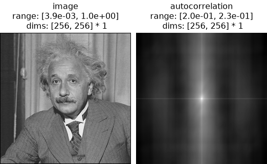
>>> import plenoptic as po
>>> import torch
>>> img = po.data.einstein()
>>> ac = po.process.autocorrelation(img)
>>> po.plot.imshow([img, ac], title=["image", "autocorrelation"])
<PyrFigure...>

(png, hires.png, pdf)

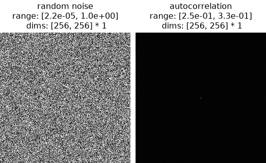
If we start from random noise, we do not see the correlation structure that is found in natural images:

>>> random_img = torch.rand(size=(1, 1, 256, 256))
>>> ac_noise = po.process.autocorrelation(random_img)
>>> po.plot.imshow(
...     [random_img, ac_noise], title=["random noise", "autocorrelation"]
... )
<PyrFigure...>

(png, hires.png, pdf)

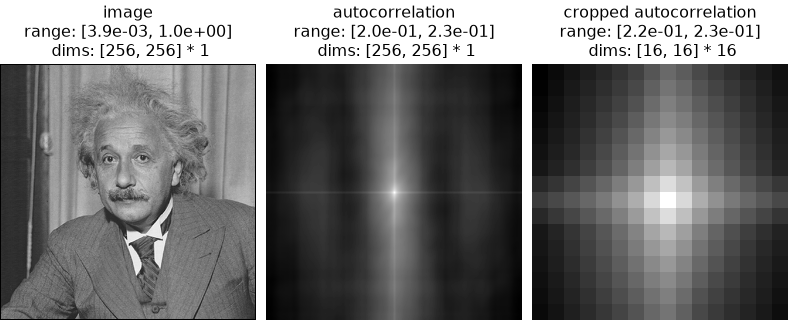
Plenoptic models typically do not use the full autocorrelation, but rather the first couple shifts only. Using a combination of this function and center_crop, that is easily achieved:

>>> ac_cropped = po.process.center_crop(ac, 16)
>>> po.plot.imshow(
...     [img, ac, ac_cropped],
...     title=["image", "autocorrelation", "cropped autocorrelation"],
... )
<PyrFigure...>

(png, hires.png, pdf)